Analysis of simulations with RoGeR

In this tutorial, we will use xarray and matplotlib to load, analyze, and plot the model output. You can run these commands in IPython or a Jupyter Notebook. Just make sure to install the dependencies first:

$ pip install xarray matplotlib netcdf4 cftime

The analysis below is conducted for a single year simulation of the SVAT setup from the model gallery.

Let’s start by importing some packages:

In [1]: import xarray as xr

In [2]: from cftime import num2date

In [3]: import numpy as np

In [4]: from pathlib import Path

Set the paths to the example data:

In [5]: OUTPUT_FILES = {
   ...:     "rate": Path().absolute() / "_data" / "SVAT.rate.nc",
   ...:     "collect": Path().absolute() / "_data" / "SVAT.collect.nc",
   ...:     "maximum": Path().absolute() / "_data" / "SVAT.maximum.nc",
   ...: }
   ...: 

Most of the heavy lifting will be done by xarray, which provides a data structure and API for working with labeled N-dimensional arrays. xarray datasets automatically keep track how the values of the underlying arrays map to locations in space and time, which makes them immensely useful for analyzing model output.

Load and plot fluxes

In order to load our first output file and display its content execute the following two commands:

In [6]: ds_rate = xr.open_dataset(OUTPUT_FILES["rate"])

In [7]: ds_rate
Out[7]: 
<xarray.Dataset>
Dimensions:                (x: 1, y: 1, z: 1, t: 1, t_forc: 1,
                            timesteps_day: 144, timesteps_event_ff: 1,
                            timesteps_event_ff_p1: 2, crops: 1, cr: 2,
                            events_ff: 1, n_sas_params: 8, n_crop_types: 76,
                            n_crop_params: 23, n_lu: 25, n_sealing: 101,
                            n_slope: 10000, n_params2: 2, n_params7: 7,
                            n_params9: 9, n_params13: 13, n_flowdir: 8,
                            Time: 366)
Coordinates: (12/23)
  * x                      (x) float64 0.0
  * y                      (y) float64 0.0
  * z                      (z) float64 0.0
  * t                      (t) float64 0.0
  * t_forc                 (t_forc) float64 0.0
  * timesteps_day          (timesteps_day) float64 0.0 1.0 2.0 ... 142.0 143.0
    ...                     ...
  * n_params2              (n_params2) float64 0.0 1.0
  * n_params7              (n_params7) float64 0.0 1.0 2.0 3.0 4.0 5.0 6.0
  * n_params9              (n_params9) float64 0.0 1.0 2.0 3.0 ... 6.0 7.0 8.0
  * n_params13             (n_params13) float64 0.0 1.0 2.0 ... 10.0 11.0 12.0
  * n_flowdir              (n_flowdir) float64 0.0 1.0 2.0 3.0 4.0 5.0 6.0 7.0
  * Time                   (Time) timedelta64[ns] 0 days 1 days ... 365 days
Data variables: (12/13)
    prec                   (Time, y, x) float64 ...
    aet                    (Time, y, x) float64 ...
    transp                 (Time, y, x) float64 ...
    evap_soil              (Time, y, x) float64 ...
    inf_mat_rz             (Time, y, x) float64 ...
    inf_mp_rz              (Time, y, x) float64 ...
    ...                     ...
    inf_ss                 (Time, y, x) float64 ...
    q_rz                   (Time, y, x) float64 ...
    q_ss                   (Time, y, x) float64 ...
    cpr_rz                 (Time, y, x) float64 ...
    dS                     (Time, y, x) float64 ...
    q_snow                 (Time, y, x) float64 ...
Attributes:
    date_created:      2023-02-08T11:41:11.396808
    roger_version:     0.0.1+507.gfc68f5f.dirty
    comment:           First timestep (t=0) contains initial values. Simulati...
    setup_identifier:  SVAT

# convert to datetime
In [8]: days = (ds_rate['Time'].values / np.timedelta64(24 * 60 * 60, "s"))

In [9]: date = num2date(days, units=f"days since {ds_rate['Time'].attrs['time_origin']}", calendar='standard', only_use_cftime_datetimes=False)

In [10]: ds_rate = ds_rate.assign_coords(Time=date)

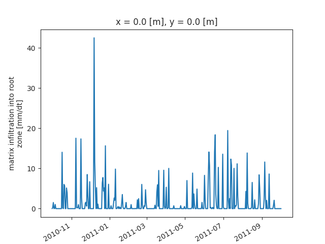
Now, we select the time series of inf_mat and plot the daily data:

In [11]: ds_rate["inf_mat_rz"].isel(x=0, y=0).plot()
Out[11]: [<matplotlib.lines.Line2D at 0x7fb6b13c3e50>]